Section 6.2 Goodness-of-Fit Tests
¶Testing Multiple Proportions.
As was the case with testing multiple means, we need to be careful how we test multiple proportions. Consider the following example.
Example 6.2.1. Testing a Statement About Multiple Proportions.
A mixed nut product claims to contain 40% peanuts, 25% hazelnuts, 15% cashews, 10% brazil nuts, and 10% other assorted nuts. You wish to test this claim by purchasing a container of mixed nuts and determining the proportion of each type of nut in your sample. How could this be done using the hypothesis tests we've seen thus far?
We could conduct five different hypothesis tests:
-
Peanuts.
\begin{align*} H_0\amp:\ p_1 = 0.40\\ H_A\amp:\ p_1 \not= 0.40 \end{align*} -
Hazelnuts.
\begin{align*} H_0\amp:\ p_2 = 0.25\\ H_A\amp:\ p_2 \not= 0.25 \end{align*} -
Cashews.
\begin{align*} H_0\amp:\ p_3 = 0.15\\ H_A\amp:\ p_3 \not= 0.15 \end{align*} -
Brazil Nuts.
\begin{align*} H_0\amp:\ p_4 = 0.10\\ H_A\amp:\ p_4 \not= 0.10 \end{align*} -
Other.
\begin{align*} H_0\amp:\ p_5 = 0.10\\ H_A\amp:\ p_5 \not= 0.10 \end{align*}
Once again, the problem we run into is that with each test, we increase the likelihood that we will make a mistake. Also, if we conduct these separate tests, we are treating the process as if it were binomial—with only two outcomes. In actuality, this process has five possible outcomes—the five types of nuts. In this section we will introduce a hypothesis test designed to check if a process with more than two possible outcomes like this has a given distribution of probabilities. Because it is designed to check how well an observed set of outcomes fits a given list of probabilities, the test is called the goodness-of-fit test.
Objectives
After finishing this section you should be able to
-
describe the following terms:
Chi-Squared Distributions
Chi-Squared Test Statistic
Degrees of Freedom for a Goodness-of-Fit Test
Expected Counts
Hypotheses for Goodness-of-Fit Tests
Multinomial Process
Observed Counts
-
accomplish the following tasks:
Identify multinomial processes
Formulate hypotheses for a goodness-of-fit test
Compute the expected counts for a goodness-of-fit test
Compute the chi-squared test statistic
Look up critical values in the chi-squared distribution table
Conduct a traditional goodness-of-fit test
Subsection 6.2.1 Multinomial Processes
¶Recall that in Section 3.2 we introduced the concept of a binomial process. The characteristics of a binomial process were defined to be:
The process consists of a fixed number of trials, each of which had only two possible outcomes: success or failure.
Each trial has the same probability of a success, \(p\text{.}\)
The trials are all independent of each other.
The result variable is the number of trials which result in successes.
Our mixed nuts example from the introduction has many of these same properties. However, the process of categorizing nuts is not binomial because each nut may fall into one of five different categories (peanut, hazelnut, etc). In a binomial process we are only allowed two possible categories: success and failure. Since our hypothesis tests for proportions are based on the assumption that we are dealing with a binomial process with only two outcomes, we need a new type of process that will work with problems such as the mixed nuts example.
Definition 6.2.2.
A multinomial process is a random process in which:
there is a fixed number of identical trials, called \(n\)
the outcomes of each trial fall into one of \(k\) possible categories
the probability of the \(i^\text{th}\) category is a fixed probability \(p_i\) with \(p_1 + p_2 + \cdots p_k = 1\text{.}\)
each of the trials is independent
The result of the process is the frequency with which each of the possible categories appear.
Let's look at a couple of examples to see if we can identify multinomial processes.
Example 6.2.3. Identifying a Multinomial Process.
A mixed nut product claims to contain 40% peanuts, 25% hazelnuts, 15% cashews, 10% brazil nuts, and 10% other assorted nuts. You wish to test this claim by purchasing a container of mixed nuts and determining the proportion of each type of nut in your sample. Is this a multinomial process?
Let's check to see if this process is multinomial by checking each property.
-
The process consists of a fixed number of identical trials.
The trials are drawing a single nut from the container. There are a fixed number of trials because there are a fixed number of nuts in the container.
-
The outcome of each trial is one of a set number of possibilities.
In this case, there are five classifications of nuts. Thus, there are only five possible outcomes: peanut, hazelnut, cashew, brazil nut, or other type of nut.
-
The probability of each category is fixed.
although we don't yet know what it is (we want to test to see if it is 40% peanuts, 25% hazelnuts, etc), the probability of getting a nut of each type is fixed (assuming there are enough nuts in the population).
-
The trials are independent.
If we consider the container of nuts we purchased to be a sample from the larger population of nuts. In this case, it is almost certain that the sample container is much smaller than (less than 5% of) the population of nuts in the packing facility.
Because each of the four properties is true, this is a multinomial process.
Example 6.2.4. Identifying When a Process is Not Multinomial.
A process consists of drawing marbles from an urn containing 1000 red marbles, 500 blue marbles, and 250 green marbles without replacement. Marbles are drawn until two green marbles have been observed. Is this a multinomial process?
This process violates the very first condition. There is no fixed number of times that we draw a marble. If our first two marbles are green, we will stop at \(n = 2\) draws. On the other hand, it could take us hundreds of draws before we see two green marbles. Because there is not a set number of trials, this is not a multinomial process.
Checkpoint 6.2.7.
Suppose that a certain gym membership comes with a “bonus feature” of either four massage sessions, four sessions with a personal trainer, or free energy drinks at the juice bar. One hundred people sign up for the gym membership, and their “bonus feature” selection is recorded.
Question: is this a multinomial process?
Yes
Checkpoint 6.2.8.
Suppose that a certain gym membership comes with a “bonus feature” of either four massage sessions, four sessions with a personal trainer, or free energy drinks at the juice bar. People are signed up until a total of at least 20 individuals have chosen each “bonus feature” and the number of individuals it took to reach that mark is recorded.
Question: is this a multinomial process?
No
Subsection 6.2.2 Formulating Hypotheses
¶A goodness-of-fit test is used to test a claim about the probabilities in a multinomial process. That is, we specify ahead of time what we believe the probability of each of the \(k\) categories should be. We then take a sample and look at the observed probability of those categories. If they are different enough from what we claimed the probabilities should be, we conclude that our claim was wrong. Since this claim involves equality (we specify what we assume the probabilities will be), it is the null hypothesis.
Principle 6.2.9. Hypotheses for Goodness-of-Fit Tests.
In a goodness-of-fit hypothesis test, we assume that a multinomial process will have probabilities \(p_1, p_2, \ldots, p_k\text{.}\) The opposite of this claim is that at least one of the probabilities is different from what we specify. Thus, the null and alternative hypotheses are:
Null hypotheses can be phrased in one of two ways. The first is as a set probabilities, as was the case in our mixed nuts example.
Example 6.2.10. Stating Hypotheses for a Goodness-of-Fit Test Based on Given Probabilities.
A mixed nut product claims to contain 40% peanuts, 25% hazelnuts, 15% cashews, 10% Brazil nuts, and 10% other assorted nuts. You wish to test this claim by purchasing a container of mixed nuts and determining the proportion of each type of nut in your sample. What are your hypotheses?
In this problem statement, we are told what the probabilities of each outcome should be. Stating those as our null hypothesis, we get:
Another common way that the null hypothesis can be phrased is in terms of relative proportions. We could claim that the outcomes are all equally likely, that one outcome is twice as likely as another, or some similar statement.
Example 6.2.11. Stating Hypotheses for a Goodness-of-Fit Test Based on Relative Probabilities.
A politician believes that the proportion of Republicans, Democrats, and independents in a certain congressional district are equal. To test this claim, she hires a polling firm to sample 500 registered voters. They find that 183 of them are Republicans, 142 of them are Democrats, and 175 of them are independents. What should the null hypothesis be for a goodness-of-fit test of the politician's claim?
In this case, the claim is that all three political parties are equally likely. If the probability of one of them is called \(x\text{,}\) then stating they are equal and recognizing that their probabilities have to sum to one gives us the following equation.
If we solve that for \(x\text{,}\) we find that \(x = \frac{1}{3}\text{.}\) Thus, our null and alternative hypothesis should be:
Checkpoint 6.2.14.
A farmer believes that in any given growing season, the probability of having a bumper crop, an average crop, or a low-yield crop is the same. He wishes to conduct a goodness-of-fit test to check this claim.
Question: what should his null hypothesis be?
\(H_0:\ p_1 = p_2 = p_3 = \frac{1}{3}\)
Checkpoint 6.2.15.
A business man believes that 60% of his customers find him through referrals, 30% through advertising, and 10% are walk-ins. He wishes to test this claim by collecting a sample of customers and seeing how well their answers to the question “how did you find our business” matches these percents.
Question: what should his null hypothesis be?
\(H_0:\ p_1 = 0.6, \quad p_2 = 0.3, \quad p_3 = 0.1\)
Subsection 6.2.3 Observed and Expected Counts
¶In a goodness-of-fit test, our goal is to compare what happens in a sample drawn from the population being studied with what we expected to happen based on the null hypothesis. The result of the sample we draw will be a list of frequencies, or counts, for each category.
Definition 6.2.16.
The number of times in a process that each category of outcome occurred are together called the observed counts for that category.
Our null hypothesis tells us what we expect the probability of each category to be. In order to compare these expected outcomes, we must convert these probabilities into expected counts. We can then compare the counts that we observed with the counts that we expected. To compute the expected counts for each category, we use the following procedure.
Theorem 6.2.17. Expected Counts.
The expected count for category \(i\) in a multinomial process is \(n\times p_i\text{,}\) where \(n\) is the total number of trials and \(p_i\) is the probability of the \(i^\text{th}\) category according to the null hypothesis.
To see how these are computed, consider the following examples.
Example 6.2.18. Finding Expected Counts Based on Given Probabilities.
A mixed nut product claims to contain 40% peanuts, 25% hazelnuts, 15% cashews, 10% Brazil nuts, and 10% other assorted nuts. You wish to test this claim by purchasing a container of mixed nuts and determining the proportion of each type of nut in your sample. The following number of each type of nuts were observed. Find the expected counts for this problem.
| Nut | Peanut | Hazelnut | Cashews | Brazil Nuts | Other |
| Observed: | 156 | 96 | 42 | 28 | 33 |
The values above are the observed counts. To find the expected counts, we multiply the total number of trials—in this case, the total number of nuts—by the probabilities of each outcome according to the null hypothesis. Recall that the null hypothesis was:
Putting this together with the counts above in tabular form gives the following table.
| Category | Observed | Expected |
| Peanut | 156 | \(0.40(355) = 142\) |
| Hazelnut | 96 | \(0.25(355) = 88.75\) |
| Cashew | 42 | \(0.15(355) = 53.25\) |
| Brazil Nut | 28 | \(0.10(355) = 35.5\) |
| Other | 33 | \(0.10(355) = 35.5\) |
| Total: | 355 | 355 |
Note that the expected counts are not necessarily whole numbers. This is because these “expected” counts are, much like the expected value, averages. Therefore they may not be numbers that can actually be observed. However, when we add together the expected counts, the total must be the same (less any rounding errors) as the observed counts. Let's look at another example.
Example 6.2.21. Finding Expected Counts Based on Relative Probabilities.
A politician believes that the proportion of Republicans, Democrats, and independents in a certain congressional district are equal. To test this claim, she hires a polling firm to sample 500 registered voters. They find that 183 of them are Republicans, 142 of them are Democrats, and 175 of them are independents. What should the null hypothesis be for a goodness-of-fit test of the politician's claim?
As we noted last time, the null hypothesis is that the probability for each political party is \(\frac{1}{3}\text{.}\) Placing the above information into a table as we did in the last example, yields the following table.
| Category | Observed | Expected |
| Republican | 179 | \(\frac{1}{3}(500) \approx 166.67\) |
| Democrats | 146 | \(\frac{1}{3}(500) \approx 166.67\) |
| Independents | 175 | \(\frac{1}{3}(500) \approx 166.67\) |
| Total: | 500 | 500.01 |
In the above example, we got a total of 500.01 for the expected counts because we rounded the fraction \(\frac{500}{3}\) to \(166.67\text{.}\)
Checkpoint 6.2.25.
In a goodness of fit test of the null hypothesis:
the following observed counts were collected.
| Category | Frequency |
| 1 | 34 |
| 2 | 68 |
| 3 | 27 |
Question: what is the expected count for category 2? Round your answer to one decimal place.
64.5
Checkpoint 6.2.27.
In a goodness of fit test of the null hypothesis:
the following observed counts were collected.
| Category | Frequency |
| 1 | 34 |
| 2 | 68 |
| 3 | 27 |
Question: what is the expected count for category 3? Round your answer to one decimal place.
25.8
Subsection 6.2.4 The \(\chi^2\)-Distribution
¶In order to measure the differences between observed and expected counts, we will need yet another distribution. This distribution is useful in hypothesis tests involving squares. As we shall see, we will use squares in the goodness-of-fit test statistic. The family of distributions, called \(\chi^2\) (pronounced /'kai skwered/) distributions, are described below.
Definition 6.2.29.
The \(\chi^2\)-distribution is a continuous probability distribution with the following properties
Like the F-distribution, the \(\chi^2\)-distribution is not symmetric, but skewed to the right.
The values of the \(\chi^2\)-distribution are non-negative (zero or larger).
The distribution is different for each degree of freedom.
As the degrees of freedom increases, the distribution becomes less skewed.
The picture below shows the members of the \(\chi^2\)-distribution family with 1, 10, and 20 degrees of freedom.

As was the case in the F-distribution, because we are always looking for large differences between observed and expected counts, we will reject the null hypothesis, which generates the expected counts, when we have large test statistics. Therefore, we will usually use right-tailed tests. However, we can use left-tailed tests to look for observed and expected counts that match too well. The following examples allow us to practice looking up critical values using the table for members of the \(\chi^2\)-distribution family.
Example 6.2.31. Using the \(\chi^2\)-Distribution Table.
Use the table below to find the following values.
The \(\chi^2\) critical value with 8 degrees of freedom at the \(\alpha = 0.05\) significance level.
The \(\chi^2\) critical value with 10 degrees of freedom at with \(0.05\) in the left tail.
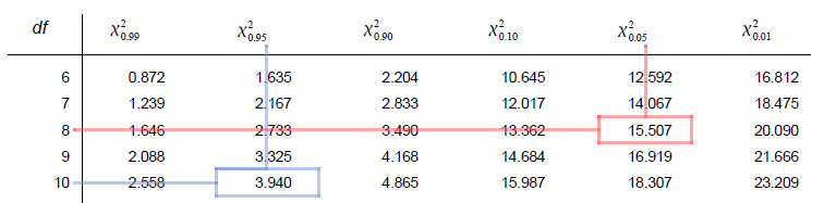
Since there are 8 degrees of freedom, and 0.05 in the right tail, we read across the 8 \(df\) row to the 0.05 column finding the critical value of 15.507. The red lines show this process.
With 10 degrees of freedom, and 0.05 in the left tail, there would be 0.95 in the right tail. Thus, we read across the 10 \(df\) row to the 0.95 column, finding a critical value of 3.940. The blue lines show this process.
Example 6.2.33. Using the \(\chi^2\)-Distribution Table In Reverse.
Use the table below to find the following values.
The probability that a \(\chi^2\) test statistic with 29 degrees of freedom is greater than 18.493.
The probability that a \(\chi^2\) test statistic with 36 degrees of freedom is less than 51.805.
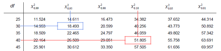
Because the table does not contain a row for 29 degrees of freedom, we round up to the closest \(df\) value that is in the table, which is 30. Looking across the \(df = 30\) row, the value 18.493 goes with a probability of 0.95 in the right tail, so the answer is 0.95. This process is outlined using the blue lines above.
As the table does not contain a row for 36 degrees of freedom, we must round up to the next lowest df in the table, which is 40. Reading across the 40 line, we find that 51.805 goes with 0.10 in the right tail. Thus, the probability of being less than 51.805 is the \(1 - 0.10 = 0.90\) in the left tail.
Checkpoint 6.2.37.
Recall that the \(\chi^2\) distribution has the following probability density curves, depending on the degrees of freedom.

Question: which of the following are properties of the chi-squared distribution?
It is skewed right
It is symmetric
It is skewed left
It has two modes
It is no negative values
As the degrees of freedom increase, it becomes more mound-shaped
(a), (e), and (f)
Checkpoint 6.2.39.
A \(\chi^2\)-distribution has 14 degrees of freedom.
Question: what critical value separates the top 10% of the data from the bottom 90%?
21.064
Subsection 6.2.5 The Test Statistic
¶To compute the test statistic for a goodness-of-fit test, our goal is to measure how far off our observed counts are from our expected counts. To do this, we want to examine the difference between observed and expected, but we don't care which is larger. Thus, we square that difference. Finally, we scale the difference by dividing by the expected counts. This is done because a difference of 10 means a lot more when only 15 were expected than it would if 100 were expected.
Theorem 6.2.40. Goodness-of-Fit Test Statistic.
The \(\chi^2\) test statistic for a goodness-of-fit test having observed counts \(O_i\) and expected counts \(E_i\) in category \(i\) is given by:
Let's look at the test statistic computation four our two examples.
Example 6.2.41. Computing the \(\chi^2\) Test Statistic for Set Probabilities.
A mixed nut product claims to contain 40% peanuts, 25% hazelnuts, 15% cashews, 10% Brazil nuts, and 10% other assorted nuts. You wish to test this claim by purchasing a container of mixed nuts and determining the proportion of each type of nut in your sample. The following number of each type of nuts were observed. Find the \(\chi^2\) test statistic.
| Nut | Peanut | Hazelnut | Cashews | Brazil Nuts | Other |
| Observed: | 156 | 96 | 42 | 28 | 33 |
To complete this task, we will add one column to the table we saw last time we worked on this example. In that column, we will compute the observed count, minus the expected count, squared and then divided by the expected count.
| Category | Observed | Expected | \(\frac{(O-E)^2}{E}\) |
| Peanut | 156 | \(0.40(355) = 142\) | \(\frac{(156-142)^2}{142} \approx 1.3081\) |
| Hazelnut | 96 | \(0.25(355) = 88.75\) | \(\frac{(96-88.75)^2}{88.75} \approx 0.5923\) |
| Cashew | 42 | \(0.15(355) = 53.25\) | \(\frac{(42-53.25)^2}{53.25} \approx 2.3768\) |
| Brazil Nut | 28 | \(0.10(355) = 35.5\) | \(\frac{(28-35.5)^2}{35.5} \approx 1.5845\) |
| Other | 33 | \(0.10(355) = 35.5\) | \(\frac{(33-35.5)^2}{35.5} \approx 0.1761\) |
| Total: | 355 | 355 | \(\chi^2_{\text{test}} \approx 5.7840\) |
Example 6.2.44. Computing the \(\chi^2\) Test Statistic for Relative Probabilities.
A politician believes that the proportion of Republicans, Democrats, and independents in a certain congressional district are equal. To test this claim, she hires a polling firm to sample 500 registered voters. They find that 183 of them are Republicans, 142 of them are Democrats, and 175 of them are independents. What is the \(\chi^2\) test statistic for a goodness-of-fit test of the politician's claim?
Again, we add a column to our table of observed and expected counts to compute the \(\chi^2\) test statistic.
| Category | Observed | Expected | \(\frac{(O-E)^2}{E}\) |
| Republican | 183 | \(\frac{1}{3}(500) \approx 166.67\) | \(\frac{(183-166.67)^2}{166.67} \approx 1.6000\) |
| Democrats | 142 | \(\frac{1}{3}(500) \approx 166.67\) | \(\frac{(142-166.67)^2}{166.67} \approx 3.6516\) |
| Independents | 175 | \(\frac{1}{3}(500) \approx 166.67\) | \(\frac{(175-166.67)^2}{166.67} \approx 0.4163\) |
| Total: | 500 | 500.01 | \(\chi^2_{\text{test}} = 5.6679\) |
Checkpoint 6.2.48.
To test the null hypothesis:
the following observed counts were collected, and the given expected counts were computed.
| Category | Observed | Expected |
| 1 | 16 | 20 |
| 2 | 33 | 40 |
| 3 | 27 | 30 |
| 4 | 24 | 30 |
Question: what is the value of \(\chi^2_{\text{test}}\) for this goodness-of-fit test?
3.525
Checkpoint 6.2.50.
To test the null hypothesis:
the following observed counts were collected, and the given expected counts were computed.
| Category | Observed | Expected |
| 1 | 19 | 25 |
| 2 | 32 | 25 |
| 3 | 28 | 25 |
| 4 | 21 | 25 |
Question: what is the value of \(\chi^2_{\text{test}}\) for this goodness-of-fit test?
4.400
Subsection 6.2.6 The Goodness-of-Fit Test
¶The goodness-of-fit test is, like any other hypothesis test, completed by comparing the test statistic from the sample to the significance level. In the case of a \(\chi^2\) test statistic, we again must use a traditional test because the table is not set up to give a p-values. That means that we need a degrees of freedom in order to look up the critical value.
Theorem 6.2.52. Degrees of Freedom for a Goodness-of-Fit Test.
The degrees of freedom for a goodness-of-fit test of a multinomial process in which there are k categories is \(df = k-1\text{.}\)
Let's finish our two examples by conducting a traditional test.
Example 6.2.53. Conducting a Goodness-of-Fit Test for Set Probabilities.
A mixed nut product claims to contain 40% peanuts, 25% hazelnuts, 15% cashews, 10% Brazil nuts, and 10% other assorted nuts. You wish to test this claim by purchasing a container of mixed nuts and determining the proportion of each type of nut in your sample. Does this sample fit the distribution claimed on the package? Use the \(\alpha = 0.05\) significance level.
| Nut | Peanut | Hazelnut | Cashews | Brazil Nuts | Other |
| Observed: | 156 | 96 | 42 | 28 | 33 |
We now put our previous work on this problem together to complete the hypothesis test. Recall that the hypotheses are:
We then construct the goodness-of-fit table below to compare the observed and expected counts and compute the test statistic.
| Category | Observed | Expected | \(\frac{(O-E)^2}{E}\) |
| Peanut | 156 | \(0.40(355) = 142\) | \(\frac{(156-142)^2}{142} \approx 1.3081\) |
| Hazelnut | 96 | \(0.25(355) = 88.75\) | \(\frac{(96-88.75)^2}{88.75} \approx 0.5923\) |
| Cashew | 42 | \(0.15(355) = 53.25\) | \(\frac{(42-53.25)^2}{53.25} \approx 2.3768\) |
| Brazil Nut | 28 | \(0.10(355) = 35.5\) | \(\frac{(28-35.5)^2}{35.5} \approx 1.5845\) |
| Other | 33 | \(0.10(355) = 35.5\) | \(\frac{(33-35.5)^2}{35.5} \approx 0.1761\) |
| Total: | 355 | 355 | \(\chi^2_{\text{test}} \approx 5.7840\) |
To make our decision, we want to compare this test statistic with the critical value that separates the top \(\alpha = 0.05\) in the right tail of a \(\chi^2\)-distribution with with \(df = 5-1 = 4\) degrees of freedom (since there are five categories of nuts) from the rest of the distribution. Looking this up in the chi-squared distribution table, we find \(\chi^2_{0.05} = 9.488\) as shown below.

Since the test statistic of 5.784 is not further into the right-tail than the critical value, we fail to reject the null hypothesis. It looks like this sample does fit the claimed distribution of nuts.
Example 6.2.57. Conducting a Goodness-of-Fit Test for Relative Probabilities.
A politician believes that the proportion of Republicans, Democrats, and independents in a certain congressional district are equal. To test this claim, she hires a polling firm to sample 500 registered voters. They find that 183 of them are Republicans, 142 of them are Democrats, and 175 of them are independents. Test this claim at the \(\alpha = 0.10\) significance level.
We stated before that the our hypothesis are:
We computed then constructed a goodness-of-fit table to compute the test statistic and found the following.
| Category | Observed | Expected | \(\frac{(O-E)^2}{E}\) |
| Republican | 183 | \(\frac{1}{3}(500) \approx 166.67\) | \(\frac{(183-166.67)^2}{166.67} \approx 1.6000\) |
| Democrats | 142 | \(\frac{1}{3}(500) \approx 166.67\) | \(\frac{(142-166.67)^2}{166.67} \approx 3.6516\) |
| Independents | 175 | \(\frac{1}{3}(500) \approx 166.67\) | \(\frac{(175-166.67)^2}{166.67} \approx 0.4163\) |
| Total: | 500 | 500.01 | \(\chi^2_{\text{test}} = 5.6679\) |
We need the critical value for the \(\alpha=0.10\) significance level in a \(\chi^2\) distribution with \(df = 3 - 1 = 2\) degrees of freedom. Looking this up in the \(\chi^2\)-distribution table, we find \(\chi^2_{0.10} = 4.605\) and sketch the picture below.

Because the test statistic is larger than the critical value (and thus further into the right tail) we must reject the null hypothesis. The three parties do not appear to have equal proportions.
Checkpoint 6.2.62.
To test the null hypothesis:
the following observed counts were collected, and the given expected counts were computed. The test statistic was then found, as shown in the table.
| Category | Observed | Expected | \(\frac{(O-E)^2}{E}\) |
| 1 | 65 | 70 | 0.357 |
| 2 | 24 | 30 | 1.200 |
| 3 | 11 | 10 | 0.100 |
| Totals: | 110 | 110 | \(\chi^2_\text{test} = 1.657\) |
Question: what conclusion should you make at the \(\alpha = 0.05\) significance level?
Fail to reject the null hypothesis.
Checkpoint 6.2.64.
To test the null hypothesis:
the following observed counts were collected, and the given expected counts were computed. The test statistic was then found, as shown in the table.
| Category | Observed | Expected | \(\frac{(O-E)^2}{E}\) |
| 1 | 61 | 70 | 1.157 |
| 2 | 18 | 30 | 4.800 |
| 3 | 21 | 10 | 12.100 |
| Totals: | 110 | 110 | \(\chi^2_\text{test} = 18.057\) |
Question: what conclusion should you make at the \(\alpha = 0.01\) significance level?
Reject the null hypothesis.