Section 4.5 Confidence Intervals for Means Using Small Samples
¶When Samples are too Small.
When we had a large sample of 30 or more, we were able to use the Central Limit Theorem to estimate the population mean based on the sample mean \(\overline{x}\) and sample standard deviation \(s\text{.}\) That is, we compute our margin of error, such as \(z_{\alpha/2}\times \frac{s}{\sqrt{n}}\text{,}\) using z-scores with a normal distribution and we freely replace \(\sigma\text{,}\) the population standard deviation, with \(s\text{,}\) the sample standard deviation. Unfortunately, if our sample size is small, we can not make these assumptions.
Consider the following situations in which this becomes a problem.
You wish to estimate the average amount of iron contained in one cubic inch of moon rock. Because of the rarity of moon rocks, you are only able to get a sample of 6 rocks to test. You can, however, assume that the amount of iron follows a normal distribution.
A widget manufacturer wishes to estimate the difference between the lifespan of a basic widget and the lifespan of a deluxe widget. Because this test destroys the widget, and widgets are expensive, they must use a small sample of 14 of each type of widget. The lifespan of a widget is known to follow a normal distribution.
Even though the underlying distributions are normal, because we do not know \(\sigma\text{,}\) the methods from the previous sections in this chapter will not work in these situations. In this lesson we will introduce a new distribution which will allow us to work with small samples such as those described here, assuming that the distribution of the individual values in the population is normal.
Objectives
After finishing this section you should be able to
-
describe the following terms:
Degrees of Freedom for a Single Sample Student's t-Distribution
Degrees of Freedom for a Two Sample Student's t-Distribution
Pooled Variance
Small Sample Confidence Interval for a Population Mean
Small Sample Confidence Interval for the Difference Between Means
Student's t-Distribution
-
accomplish the following tasks:
Describe the properties of the Student's t-Distribution
Look up critical values in the t-distribution table
Find the margin of error for a small sample estimate of a single population mean or the difference between two means
Find a confidence interval for a small sample mean or the difference between two small sample means
Subsection 4.5.1 Student's t Distribution
¶To construct confidence intervals for means based on small samples drawn from normal populations, we must either know what \(\sigma\) is, or we must come up with a new distribution. It is unreasonable, as mentioned previouly, to know the population standard deviation when we are trying to estimate the population mean. We therefore introduce a new distribution.
This distribution is actually an entire family of distributions, one for each possible sample size less than 30. It is called the student's t-distribution because the author, who worked for a brewery, was not allowed to publish his results so as to keep these tools away from competing breweries. The author believed, however, that this information should be shared and so he published it under the pen-name “Student.”
Definition 4.5.1.
The student's t-distribution is the name given to the distribution of the variable \(t\) based on a random sample of size \(n\) with mean \(\overline{x}\) and standard deviation \(s\text{,}\) drawn from a normal population. The variable \(t\) is:
Note that the formula for \(t\) looks a lot like the the formula for the standard normal variable \(z\text{.}\) The main difference is that we are using \(s\text{,}\) the sample standard deviation, instead of \(\sigma\text{,}\) the population standard deviation. This is no longer just an “approximation,” which we could get away with in larger samples. This is now the exact value of \(t\text{.}\) So what does the distribution of \(t\) look like? Below is a graph of the normal distribution, along with the distribution of \(t\) for several different sample sizes.

Notice that the normal distribution, in black, is the tallest with the shortest tails. The t-distributions look very similar, but they are shorter and have thicker tails. The notation \(df\) stands for degrees of freedom. This is a measure of how big the sample size is—although it is not exactly equal to the sample size. The bigger the degrees of freedom, the more closely the student's t-distribution matches the normal distribution. In fact, when the degrees of freedom is 30 or more, the student's t-distribution will be so close to the normal distribution that we can just use the normal distribution critical values.
Because there are so many different student's t-distributions, the table that we use to look up critical values looks somewhat different than the normal distribution table. We list the five most common right-tail areas across the top:
We list the different degrees of freedom from 1 to 30 down the left side. The critical values, or t-scores, are found in the body of the table in the row corresponding to the appropriate degrees of freedom and the column corresponding to the area in the right tail. Note that there are no negative critical values listed in the table, and no left-tail probabilities. This is because we can use symmetry, just as in the normal distribution, to look up those critical values based on the positive values in the table.
Example 4.5.3. Looking Up Critical Values in the Student' t-Distribution.
Use the portion of the t-table shown below to find the value of t that:
has nine degrees of freedom and separates the top 2.5% of data from the bottom 97.5% of data.
has seven degrees of freedom and is the positive critical value at the 99% confidence level.
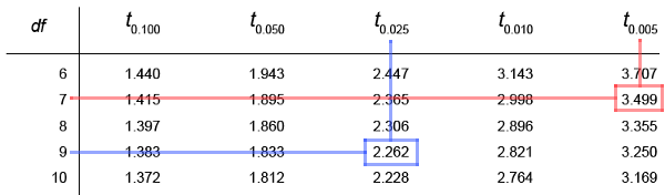
Since there are nine degrees of freedom, we go to the row with \(df=9\text{.}\) Then, since we want 2.5%, or \(0.025\text{,}\) in the right tail, we go over to \(t_{0.025}\text{.}\) The blue box shows the resulting t-score critical value is \(2.262\text{.}\)
This time there are seven degrees of freedom, and we want \(0.005\) in the right tail, since this is half of \(1 - 0.99 = 0.01\text{.}\) The red box shows us the critical value \(t_{\alpha/2} = 3.499\text{.}\)
Now some negative examples.
Example 4.5.5. Finding Negative Critical Values from the Student' t-Distribution.
Use the portion of the t-table shown below to find the value of \(t\) that:
has 12 degrees of freedom and separates the left tail with area 0.05 from the rest of the graph.
has 14 degrees of freedom and is the negative critical value at the 98% confidence level.
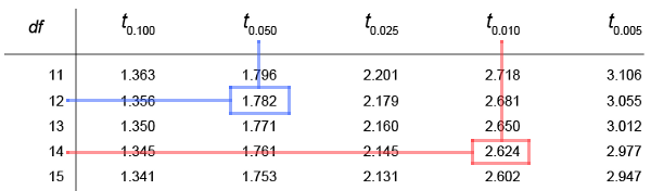
Going to the \(df=12\) row, we move over the the column labeled \(t_{0.050}\text{.}\) The entry in the blue box is the t-score separating the body of the data from the right tail with an area of \(0.05\text{.}\) Since we want the left tail, we just change the sign to get a t-score of \(-1.782\text{.}\)
The red lines show the entry with \(df=14\) and a right-tail probability of \(0.010\text{.}\) Since we want the negative critical value, we switch the sign to get \(t_{\alpha/2} = -2.624\text{.}\)
Checkpoint 4.5.9.
You wish to look up the positive critical t-value in the student's t-distribution that has 11 degrees of freedom and goes with a confidence level of 98%.
Question: what is this critical value?
2.718
Checkpoint 4.5.10.
You wish to find the negative critical value that goes with a 95% lower confidence bound. There are \(df = 17\) degrees of freedom.
Question: what is the critical t-value in this situation?
-1.740
Subsection 4.5.2 Single Population Mean
¶The process for building a confidence interval for a population mean based on a small sample should be very familiar. Aside from using the t-distribution to look up critical values, it is in fact exactly the same as what was done for large-sample estimation. Below you will find the formula for this confidence interval.
Theorem 4.5.11. Small Sample Confidence Interval for a Population Mean.
The \((1-\alpha)100\%\) small sample confidence interval for a population mean based on a sample of size \(n\) taken from a normal population with sample mean \(\overline{x}\) and standard deviation \(s\) is given by:
where \(t_{\alpha/2}\) is a critical value taken from the student's t-distribution with \(df=n-1\) degrees of freedom.
This confidence interval is still made up of a point estimate plus-or-minus a margin of error. Again the sample mean is the point estimate, and the margin of error is based on the critical value t-score for a given confidence level and degrees of freedom. Note that we do need to assume that the distribution whose mean we are trying to estimate is normal.
Example 4.5.12. Finding a Confidence Interval for a Small Sample Mean.
You wish to estimate the average amount of iron contained in one cubic inch of moon rock. Because of the rarity of moon rocks, you are only able to get a sample of 6 rocks to test. You can, however, assume that the amount of iron follows a normal distribution. Your tests show that in these six rocks, there is a mean of \(\overline{x} = 2.4\) grams per cubic inch with a standard deviation of 0.35 grams per cubic inch. Use this information to construct a 99% confidence interval for the amount of iron contained in one cubic inch of moon rock.
From the t-distribution table with \(df = 6-1 = 5\) and \(0.005\) in the right tail, the critical value is \(t_{0.005} = 4.032\text{.}\) Plugging this into the formula for the confidence interval, we get:
Adding and subtracting gives us the following confidence interval.
Example 4.5.13. Finding an Upper Confidence Bound for a Small Sample Mean.
The salaries from the top 10 business executives in your state have a mean value of $84 million with a standard deviation of $12.4 million. Assuming that the salaries of top business executives are normally distributed, find a 95% upper confidence bound for the average salary of a top business executive in your state.
Because this is an upper confidence bound, we want the entire \(\alpha = 0.05\) in the right tail. That means, we want to find \(t_{0.05}\) with \(n - 1 = 10 - 1 = 9\) degrees of freedom. Using the value \(t_{0.05} = 1.833\) found in the t-distribution table, we get the following upper bound.
Therefore, we conclude that we are 95% confident that the average salary of top executives in your state is less than $91.188 million.
Checkpoint 4.5.17.
To estimate the mean weight of a blue whale, you somehow manage to measure 6 different blue whales and find a sample mean of \(\overline x= 297,451\) pounds with a standard deviation of \(s = 9,542.5\) pounds.
Question: what is the 99% confidence interval for the true average weight of a blue whale?
\(281,744 \lt \mu \lt 313,158\)
Checkpoint 4.5.18.
In order to estimate the number of times a week that an NBA player eats at home, a sample of 16 NBA players are interviewed and the mean number of times is found to be 6.8 with a standard deviation of 2.8 days.
Question: what is the 95% confidence interval for the true average number of times a week that an NBA player eats at home?
\(5.308 \lt \mu \lt 8.292\)
Subsection 4.5.3 Difference Between Means
¶When using large samples to estimate the difference between two population means, we found that we could use the following for the standard deviation of the sampling distribution for the difference between the sample means.
As long as both samples contain 30 or more individuals, we can approximate \(\sigma_1 \approx s_1\) and \(\sigma_2 \approx s_2\) and the distribution of \(\overline{x}_1 - \overline{x}_2\) will be normal with this standard deviation. Unfortunately, for samples of size less than 30, the approximation using sample means will not work, and it will not even have a t-distribution.
It turns out that in order to get critical values for the difference between two sample means, we have to make one more assumption. We have to assume that the two populations from which we are sampling have the same variance and therefore standard deviation, so \(\sigma_1^2\) and \(\sigma_2^2\) are the same. However when we draw samples we can not expect that they will come out with exactly the same variance. To get as accurate an estimate of what that single variance is, we must combine the variances of our two samples into a pooled variance as shown below.
Definition 4.5.19. Pooled Variance.
If samples of sizes \(n_1\) and \(n_2\) with variances \(s_1^2\) and \(s_2^2\) respectively are drawn from independent populations with a common variance \(\sigma^2\text{,}\) then the pooled estimate for this variance based on these samples is:
We can then use this pooled variance in place of both \(\sigma_1^2\) and \(\sigma_2^2\) in the standard error formula above to get the following confidence interval formula for small samples.
Theorem 4.5.20. Small Sample Confidence Interval for the Difference Between Means.
The \((1-\alpha)100\%\) small sample confidence interval for the difference between population means, \(\mu_1 - \mu_2\text{,}\) based on two independent samples of sizes \(n_1\) and \(n_2\) drawn from normal populations with a common variance, estimated by the pooled variance \(s^2\text{,}\) and having sample means \(\overline{x}_1\) and \(\overline{x}_2\) is:
where \(t_{\alpha/2}\) is taken from a student's t-distribution with \(n_1 + n_2 - 2\) degrees of freedom.
Notice that the degrees of freedom depends on the size of the two samples used to construct the confidence interval. It can also be seen in the denominator of the pooled variance estimate, in case you forget. Now let's take a look at several examples in which we must make use of these formulas.
Example 4.5.21. Finding a Confidence Interval for a Difference Between Small Sample Means.
A widget manufacturer wishes to estimate the difference between the lifespan of a basic widget and the lifespan of a deluxe widget, both of which are known to have a normal distribution. Two samples are taken and the following information is gathered. Find the 90% confidence interval for the difference between the mean lifespan of a basic widget and a deluxe widget.
| Sample Size | Sample Mean | Sample StDev | |
| Basic | \(n_1 = 14\) | \(\overline{x}_1 = 742\) days | \(s_1 = 42.1\) days |
| Deluxe | \(n_2 = 12\) | \(\overline{x}_2 = 951\) days | \(s_2 = 39.6\) days |
We first find the critical value for this confidence interval. A 90% confidence interval will have an area of \(0.05\) in each tail. The degrees of freedom is \(df = 14 + 12 - 2 = 24\text{.}\) This gives us a critical value \(t_{0.050} = 1.711\text{.}\)
Our pooled variance is:
Finally, we put this all together into our confidence interval formula.
Adding and subtracting gives the following confidence interval.
Example 4.5.23. Finding an Lower Confidence Bound for a Difference Between Two Small Sample Means.
A researcher wishes to estimate the difference between achievement test scores in affluent neighborhoods and low-income neighborhoods using the few test scores which he has collected from parents. To assist in this he is going to construct a 99% lower confidence bound for the mean test scores in affluent neighborhoods and mean test scores in low-income neighborhoods. The following data is collected.
| Sample Size | Sample Mean | Sample StDev | |
| Affluent | \(n_1 = 16\) | \(\overline{x}_1 = 94\) | \(s_1^2 = 71\) |
| Low-Income | \(n_2 = 19\) | \(\overline{x}_2 = 73\) | \(s_2^2 = 185\) |
Again we start by finding the critical value. The degrees of freedom in this case is \(df = 16 + 19 - 2 = 33\text{.}\) For a 99% lower confidence bound, we want \(0.01\) in the left tail, so the critical value is \(-t_{0.010} = -2.326\text{.}\)
The pooled variance is:
We use the formula for a confidence interval, but only subtract the margin of error to find the lower confidence bound.
We are therefore 99% confident that students in the affluent neighborhoods score at least 11.9 points better on standardized tests than do those in low-income neighborhoods.
Checkpoint 4.5.28.
To estimate the difference between the time it takes fire and police to respond to emergencies, you randomly select several recent emergencies and collect the following data.
| Sample Size | Mean Time | StDev Time | |
| Fire | \(n_1 = 12\) | \(\overline{x}_1 = 6.3\) minutes | \(s_1 = 1.46\) minutes |
| Police | \(n_2 = 8\) | \(\overline{x}_2 = 5.2\) minutes | \(s_2 = 2.33\) minutes |
Question: what is the 99% confidence interval for the difference between the average response times for fire and police?
\(-1.327 \lt \mu_1-\mu_2 \lt 3.527\)
Checkpoint 4.5.30.
You wish to estimate the difference between the number of Skittles in a regular sized bag and the number of M&M's in a regular sized bag. To do this, you collect the following information:
Number of Skittles: 62, 67, 64, 71, 59, 63
Number of M&M's: 58, 63, 55, 59, 42
Using this data you compute the sample means and standard deviations shown below.
| Sample Size | Mean | StDev | |
| Skittles | 6 | 64.33 | 4.18 |
| M&M's | 5 | 55.4 | 8.02 |
Question: what is the 95% confidence interval for the difference between the mean number of Skittles and M&M's in a regular sized bag?
\(0.454 \lt \mu_1 - \mu_2 \lt 17.406\)
Subsection 4.5.4 When to Use the Student's t-Distribution
¶Since the formulas we've seen in this lesson are a lot like the formulas for a normal distribution, trying to decide which type of critical values to use can be difficult. The following rules of thumb should help you to choose the correct type of distribution to use.
-
For estimating means:
If the sample size or sizes are greater than 30, we should use the normal distribution techniques from previous sections.
-
If any sample size is less than 30 and the population has a normal distribution, then:
If we somehow know the population standard deviation, we should still use the normal distribution techniques from previous sections.
If the population standard deviation is not known, then we must use the t-distribution techniques from this section.
-
For estimating proportions:
If each of \(n\times p_1\text{,}\) \(n\times q_1\text{,}\) and if necessary, \(n\times p_2\) and \(n\times q_2\) are all greater than 5, then we can use the normal techniques seen in previous sections.
Notice that if we have small samples and we do not know that the population has a normal distribution, then none of the above apply. Also, if we have a proportion in which one of the products is not greater than 5, none of the above apply. In these cases, will not be able to perform estimation using the tools described in this text.
Example 4.5.32. Determining Which Distribution to Use.
For each of the situations below, determine what distribution we should use to construct a confidence interval: normal, t-distribution, or neither.
The proportion of a population with a given characteristic is to be approximated using a sample of 40 individuals, 12 of which have the desired characteristic.
A population mean is to be estimated using a sample of size 50. The standard deviation of the population is not known, and the population may not be normal.
The difference between proportions in two independent populations is to be estimated, but only one individual in the second sample had the desired characteristic.
The difference between two population means is to be estimated using samples of size 20 and 40. The population distributions are known to be normal.
Since \(n\times p = 12\) and \(n\times q = 28\text{,}\) we can use the normal distribution for our critical values.
Because the sample size is 30 or more, we can use the normal distribution and approximate \(\sigma\) with the sample standard deviation.
Since \(n\times p = 1\) for one of the two samples, we can not use the normal distribution. We will unfortunately not be able to build a confidence interval for this difference with the tools we have available.
Because one of the two samples is smaller than 30, we must use small sample techniques and the t-distribution to construct this confidence interval.
Checkpoint 4.5.34.
Consider the following estimation tasks.
Constructing a confidence interval for a single population proportion in which \(n\times p\) and \(n\times q\) are both greater than five.
Constructing a confidence interval for a single mean in which the population has a normal distribution, and the sample size is \(n = 100\text{.}\)
Constructing a confidence interval for a single mean in which the population has a normal distribution, and the sample size is \(n = 20\text{.}\)
Constructing a confidence interval for a difference between means in which the two populations have normal distributions, but different standard deviations, using samples of size 10.
Question: which distribution, if any, can be used to construct these intervals
normal
normal
t-distribution
none
Checkpoint 4.5.35.
Consider the following estimation tasks.
Constructing a confidence interval for a single population mean in which the population has a uniform distribution and the sample size is n = 10.
Constructing a confidence interval for a difference between means in which the populations have a normal distribution and the sample sizes are 100 and 150.
Constructing a confidence interval for the difference between proportions where \(n\times p_1 = 1\text{.}\)
Constructing a confidence interval for the difference between means when the sample sizes are 10 and 15, and the populations have a normal distribution with equal variances.
Question: which distribution, if any, can be used to construct these intervals
none
normal
none
t-distribution